Exploring & working with data in R and tidyverse
Exploring data in R
In this lesson, we'll spend time unpacking the basic data structures in R that we breezed past in our previous lesson. Then, we'll go over how to read in data and manipulate it in tidyverse.
Note that this lesson has been modified from The Carpentries alternative version of the R Ecology lesson. Parts are reproduced in full, but the major changes were included to shorten the lesson to 60 minutes.
The data.frame
In the previous lesson, we created visualizations from the complete_old data, but we did not talk much about what this complete_old thing is.
During this lesson, we'll cover how R represents, uses, and stores data.
To start out, launch a fresh RStudio application window and load the two packages we'll work with during this lesson.
library(tidyverse)
library(ratdat)
The complete_old data is stored in R as a data.frame, which is the most common way that R represents tabular data (data that can be stored in a table format, like a spreadsheet).
We can check what complete_old is by using the class() function:
class(complete_old)
## [1] "data.frame"
We can view the first few rows with the head() function, and the last few rows with the tail() function:
head(complete_old)
##   record_id month day year plot_id species_id sex hindfoot_length weight
## 1         1     7  16 1977       2         NL   M              32     NA
## 2         2     7  16 1977       3         NL   M              33     NA
## 3         3     7  16 1977       2         DM   F              37     NA
## 4         4     7  16 1977       7         DM   M              36     NA
## 5         5     7  16 1977       3         DM   M              35     NA
## 6         6     7  16 1977       1         PF   M              14     NA
##         genus  species   taxa                plot_type
## 1     Neotoma albigula Rodent                  Control
## 2     Neotoma albigula Rodent Long-term Krat Exclosure
## 3   Dipodomys merriami Rodent                  Control
## 4   Dipodomys merriami Rodent         Rodent Exclosure
## 5   Dipodomys merriami Rodent Long-term Krat Exclosure
## 6 Perognathus   flavus Rodent        Spectab exclosure
tail(complete_old)
##       record_id month day year plot_id species_id sex hindfoot_length weight
## 16873     16873    12   5 1989       8         DO   M              37     51
## 16874     16874    12   5 1989      16         RM   F              18     15
## 16875     16875    12   5 1989       5         RM   M              17      9
## 16876     16876    12   5 1989       4         DM   M              37     31
## 16877     16877    12   5 1989      11         DM   M              37     50
## 16878     16878    12   5 1989       8         DM   F              37     42
##                 genus   species   taxa        plot_type
## 16873       Dipodomys     ordii Rodent          Control
## 16874 Reithrodontomys megalotis Rodent Rodent Exclosure
## 16875 Reithrodontomys megalotis Rodent Rodent Exclosure
## 16876       Dipodomys  merriami Rodent          Control
## 16877       Dipodomys  merriami Rodent          Control
## 16878       Dipodomys  merriami Rodent          Control
Refresher on named arguments & argument order
We used these functions with just one argument, the object complete_old, and we didn't give the argument a name, like we often did with ggplot2.
In R, a function's arguments come in a particular order, and if you put them in the correct order, you don't need to name them.
In this case, the name of the argument is x, so we can name it if we want, but since we know it's the first argument, we don't need to.
To learn more about a function, you can type a ? in front of the name of the function, which will bring up the official documentation for that function:
?head
Some arguments are optional.
For example, the n argument in head() specifies the number of rows to print.
It defaults to 6, but we can override that by specifying a different number:
head(complete_old, n = 10)
head(complete_old, 10)
head(n = 10, x = complete_old)
As we have already done, we can use str() to look at the structure of an object:
str(complete_old)
## 'data.frame':    16878 obs. of  13 variables:
##  $ record_id      : int  1 2 3 4 5 6 7 8 9 10 ...
##  $ month          : int  7 7 7 7 7 7 7 7 7 7 ...
##  $ day            : int  16 16 16 16 16 16 16 16 16 16 ...
##  $ year           : int  1977 1977 1977 1977 1977 1977 1977 1977 1977 1977 ...
##  $ plot_id        : int  2 3 2 7 3 1 2 1 1 6 ...
##  $ species_id     : chr  "NL" "NL" "DM" "DM" ...
##  $ sex            : chr  "M" "M" "F" "M" ...
##  $ hindfoot_length: int  32 33 37 36 35 14 NA 37 34 20 ...
##  $ weight         : int  NA NA NA NA NA NA NA NA NA NA ...
##  $ genus          : chr  "Neotoma" "Neotoma" "Dipodomys" "Dipodomys" ...
##  $ species        : chr  "albigula" "albigula" "merriami" "merriami" ...
##  $ taxa           : chr  "Rodent" "Rodent" "Rodent" "Rodent" ...
##  $ plot_type      : chr  "Control" "Long-term Krat Exclosure" "Control" "Rodent Exclosure" ...
One thing we didn't cover previously when looking at the output of the str() function was the preponderance of $ -- each variable is preceded by a $.
The $ is an operator that allows us to select individual columns from a data.frame.
Like functions and their arguments, we can use tab-completion after $ to select which variable you want from a given data.frame.
For example, to get the year variable, we can type complete_old$ and then hit Tab.
We get a list of the variables that we can move through with up and down arrow keys. Hit Enter when you reach year, which should finish this code:
complete_old$year
This prints the values of the year column to the console.
Vectors: the building block of data
You might have noticed that our last result looked different from when we printed out the complete_old data.frame itself.
That's because it is not a data.frame, it is a vector.
A vector is a 1-dimensional series of values, in this case a vector of numbers representing years.
Data.frames are made up of vectors; each column in a data.frame is a vector. Vectors are the basic building blocks of all data in R. Basically, everything in R is a vector, a bunch of vectors stitched together in some way, or a function.
There are 4 main types of vectors (also known as atomic vectors):
-
"character"for strings of characters, like ourgenusorsexcolumns. Each entry in a character vector is wrapped in quotes. In other programming languages, this type of data may be referred to as "strings". -
"integer"for integers. All the numeric values incomplete_oldare integers. You may sometimes see integers represented like2Lor20L. TheLindicates to R that it is an integer, instead of the next data type,"numeric". -
"numeric", aka"double", vectors can contain numbers including decimals. Other languages may refer to these as "float" or "floating point" numbers. -
"logical"forTRUEandFALSE, which can also be represented asTandF. In other contexts, these may be referred to as "Boolean" data.
Vectors can only be of a single type. Since each column in a data.frame is a vector, this means an accidental character following a number, like 29, can change the type of the whole vector.
To create a vector from scratch, we can use the c() function, putting values inside, separated by commas.
c(1, 2, 5, 12, 4)
## [1] 1 2 5 12 4
As you can see, those values get printed out in the console, just like with complete_old$year.
To store this vector so we can continue to work with it, we need to assign it to an object.
num <- c(1, 2, 5, 12, 4)
You can check what kind of object num is with the class() function.
class(num)
## [1] "numeric"
We see that num is a numeric vector.
Let's try making a character vector:
char <- c("apple", "pear", "grape")
class(char)
## [1] "character"
Remember that each entry, like "apple", needs to be surrounded by quotes, and entries are separated with commas.
If you do something like "apple, pear, grape", you will have only a single entry containing that whole string.
Finally, let's make a logical vector:
logi <- c(TRUE, FALSE, TRUE, TRUE)
class(logi)
## [1] "logical"
Challenge 1: Coercion
Since vectors can only hold one type of data, something has to be done when we try to combine different types of data into one vector.
- What type will each of these vectors be? Try to guess without running any code at first, then run the code and use
class()to verify your answers.
num_logi <- c(1, 4, 6, TRUE)
num_char <- c(1, 3, "10", 6)
char_logi <- c("a", "b", TRUE)


tricky <- c("a", "b", "1", FALSE)
Challenge solution
class(num_logi)
## [1] "numeric"
class(num_char)
## [1] "character"
class(char_logi)
## [1] "character"
class(tricky)
## [1] "character"
R will automatically convert values in a vector so that they are all the same type, a process called coercion.
- How many values in
combined_logicalare"TRUE"(as a character)?
combined_logical <- c(num_logi, char_logi)
Challenge solution
combined_logical
## [1] "1" "4" "6" "1" "a" "b" "TRUE"
class(combined_logical)
## [1] "character"
Only one value is "TRUE".
Coercion happens when each vector is created, so the TRUE in num_logi becomes a 1, while the TRUE in char_logi becomes "TRUE".
When these two vectors are combined, R doesn't remember that the 1 in num_logi used to be a TRUE, it will just coerce the 1 to "1".
- Now that you've seen a few examples of coercion, you might have started to see that there are some rules about how types get converted. There is a hierarchy to coercion. Can you draw a diagram that represents the hierarchy of what types get converted to other types?
Challenge solution
logical → integer → numeric → characterLogical vectors can only take on two values: TRUE or FALSE. Integer vectors can only contain integers, so TRUE and FALSE can be coerced to 1 and 0.
Numeric vectors can contain numbers with decimals, so integers can be coerced from, say, 6 to 6.0 (though R will still display a numeric 6 as 6.).
Finally, any string of characters can be represented as a character vector, so any of the other types can be coerced to a character vector.
Coercion most often happens when combining vectors when they contain different data types or reading data into R where a stray character may change an entire numeric vector into a character vector.
Using the class() function can help confirm an object's class meets your expectations, particularly if you are running into confusing error messages.
Missing data
R represents missing data as NA, without quotes, in vectors of any type.
The NA signals to R to treat that data differently than the rest of the entries in the vector.
Let's make a numeric vector with an NA value:
weights <- c(25, 34, 12, NA, 42)
By default, may R functions won't work when NA values are present; instead, if you use them they'll return NA themselves.
min(weights)
## [1] NA
This behavior protects the user from not considering missing data. If we decide to exclude our missing values, many basic math functions have an argument to remove them:
min(weights, na.rm = TRUE)
## [1] 12
Vectors as arguments
A common reason to create a vector from scratch is to use in a function argument.
For example, the quantile() function will calculate a quantile for a given vector of numeric values.
We set the quantile using the probs argument.
We also need to set na.rm = TRUE, since there are NA values in the weight column.
quantile(complete_old$weight, probs = 0.25, na.rm = TRUE)
## 25%
##  24
Now we get back the 25% quantile value for weights.
However, we often want to know more than one quantile.
Luckily, the probs argument is vectorized, meaning it can take a whole vector of values.
Let's try getting the 25%, 50% (median), and 75% quantiles all at once.
quantile(complete_old$weight, probs = c(0.25, 0.5, 0.75), na.rm = TRUE)
## 25% 50% 75%
##  24  42  53
Other data tyes in R
We have now seen vectors in a few different forms: as columns in a data.frame and as single vectors. However, they can be manipulated into lots of other shapes and forms. Some other common forms are:
- matrices
- 2-dimensional numeric representations
- arrays
- many-dimensional numeric
- lists
- lists are very flexible ways to store vectors
- a list can contain vectors of many different types and lengths
- an entry in a list can be another list, so lists can get deeply nested
- a data.frame is a type of list where each column is an individual vector and each vector has to be the same length, since a data.frame has an entry in every column for each row
- factors
- a way to represent categorical data
- factors can be ordered or unordered
- they often look like character vectors, but behave differently
- under the hood, they are integers with character labels, called levels, for each integer
We won't spend time on these data types in this lesson. If you want more information on these classes, you can read through this Software Carpentry lesson.
Working with data in R
Importing data
Up until this point, we have been working with the complete_old data.frame contained in the ratdat package.
However, you typically won't access data from an R package; it is much more common to access data files stored somewhere on your computer.
We are going to download a CSV file containing the surveys data to our computer, which we will then read into R.
Click this link to download the file: https://github.com/Arcadia-Science/arcadia-computational-training/blob/main/docs/arcadia-users-group/20231031-intro-to-r/surveys_complete_77_89.csv.
You will be prompted to save the file on your computer somewhere.
Save it in your ~/Downloads folder so that we'll all be working with the same file path.
More information on project organization and management.
For this lesson, we aren't worrying about our file and folder organization. In general, it's best practice to keep your project organized in a specific folder. The exact organization strategy will depend on the project you're doing and the tools you choose to use. For more information on how to keep your project organized, a discussion of some best practices, and strategies you can use, see the lesson Project organization and file & resource management.File paths
When we reference other files from an R script, we need to give R precise instructions on where those files are.
We do that using something called a file path.
It looks something like this: "~/Documents/Manuscripts/Chapter_2.txt".
This path would tell your computer how to get from whatever folder contains the Documents folder all the way to the .txt file.
There are two kinds of paths: absolute and relative. Absolute paths are specific to a particular computer, whereas relative paths are relative to a certain folder. For more information on fie paths and directory structures, see this lesson.
Let's read our CSV file into R and store it in an object named surveys.
We will use the read_csv function from the tidyverse's readr package.
surveys <- read_csv("~/Downloads/surveys_complete_77_89.csv")
## Rows: 16878 Columns: 13
## ── Column specification ────────────────────────────────────────────────────────
## Delimiter: ","
## chr (6): species_id, sex, genus, species, taxa, plot_type
## dbl (7): record_id, month, day, year, plot_id, hindfoot_length, weight
##
## ℹ Use `spec()` to retrieve the full column specification for this data.
## ℹ Specify the column types or set `show_col_types = FALSE` to quiet this message.
Using tab completion to solve the file path.
Typing out paths can be error prone, so we can utilize a keyboard shortcut. Just like functions and other objects in RStudio, you can use tab completion on file paths. Inside the parentheses ofread_csv(), type out a pair of quotes and put your cursor between them.
Then hit Tab.
A small menu showing your folders and files should show up.
You can use the ↑ and ↓ keys to move through the options, or start typing to narrow them down.
You can hit Enter to select a file or folder, and hit Tab again to continue building the file path.
This might take a bit of getting used to, but once you get the hang of it, it will speed up writing file paths and reduce the number of mistakes you make.
By default, the read_csv() function prints information about the files it reads to the Console.
We got some useful information about the CSV file we read in.
We can see:
- the number of rows and columns
- the delimiter of the file, which is how values are separated, a comma
"," - a set of columns that were parsed as various vector types
- the file has 6 character columns and 7 numeric columns
- we can see the names of the columns for each type
When working with the output of a new function, it's often a good idea to check the class():
class(surveys)
## [1] "spec_tbl_df" "tbl_df" "tbl" "data.frame"
Whoa! What is this thing? It has multiple classes? Well, it's called a tibble, and it is the tidyverse version of a data.frame. It is a data.frame, but with some added perks. It prints out a little more nicely, it highlights NA values and negative values in red, and it will generally communicate with you more (in terms of warnings and errors, which is a good thing).
The difference between tidyverse and base R
As we begin to delve more deeply into the tidyverse, we should briefly pause to mention some of the reasons for focusing on the tidyverse set of tools.
In R, there are often many ways to get a job done, and there are other approaches that can accomplish tasks similar to the tidyverse.
The phrase base R is used to refer to approaches that utilize functions contained in R's default packages.
We have already used some base R functions, such as str(), head(), and mean(), and we will be using more scattered throughout this lesson.
However, this lesson won't cover some functionalities in base R such as sub-setting with square bracket notation and base plotting.
You may come across code written by other people that looks like surveys[1:10, 2] or plot(surveys$weight, surveys$hindfoot_length), which are base R commands.
If you're interested in learning more about these approaches, you can check out other Carpentries lessons like the Software Carpentry Programming with R lesson.
We choose to teach the tidyverse set of packages because they share a similar syntax and philosophy, making them consistent and producing highly readable code.
They are also very flexible and powerful, with a growing number of packages designed according to similar principles and to work well with the rest of the packages.
The tidyverse packages tend to have very clear documentation and wide array of learning materials that tend to be written with novice users in mind.
Finally, the tidyverse has only continued to grow, and has strong support from Posti (the RStudio parent company), which implies that these approaches will be relevant into the future.
Manipulating data
One of the most important skills for working with data in R is the ability to manipulate, modify, and reshape data.
The dplyr and tidyr packages in the tidyverse provide a series of powerful functions for many common data manipulation tasks.
We'll start off with two of the most commonly used dplyr functions: select(), which selects certain columns of a data.frame, and filter(), which filters out rows according to certain criteria.
Between select() and filter(), it can be hard to remember which operates on columns and which operates on rows.
select() has a c for columns and filter() has an r for rows.
select()
To use the select() function, the first argument is the name of the data.frame, and the rest of the arguments are unquoted names of the columns you want:
select(surveys, plot_id, species_id, hindfoot_length)
## # A tibble: 16,878 × 3
##    plot_id species_id hindfoot_length
##      <dbl> <chr>                <dbl>
##  1       2 NL                      32
##  2       3 NL                      33
##  3       2 DM                      37
##  4       7 DM                      36
##  5       3 DM                      35
##  6       1 PF                      14
##  7       2 PE                      NA
##  8       1 DM                      37
##  9       1 DM                      34
## 10       6 PF                      20
## # ℹ 16,868 more rows
The columns are arranged in the order we specified inside select().
To select all columns except specific columns, put a - in front of the column you want to exclude:
select(surveys, -record_id, -year)
## # A tibble: 16,878 × 11
##    month   day plot_id species_id sex   hindfoot_length weight genus     species
##    <dbl> <dbl>   <dbl> <chr>      <chr>           <dbl>  <dbl> <chr>     <chr>
##  1     7    16       2 NL         M                  32     NA Neotoma   albigu…
##  2     7    16       3 NL         M                  33     NA Neotoma   albigu…
##  3     7    16       2 DM         F                  37     NA Dipodomys merria…
##  4     7    16       7 DM         M                  36     NA Dipodomys merria…
##  5     7    16       3 DM         M                  35     NA Dipodomys merria…
##  6     7    16       1 PF         M                  14     NA Perognat… flavus
##  7     7    16       2 PE         F                  NA     NA Peromysc… eremic…
##  8     7    16       1 DM         M                  37     NA Dipodomys merria…
##  9     7    16       1 DM         F                  34     NA Dipodomys merria…
## 10     7    16       6 PF         F                  20     NA Perognat… flavus
## # ℹ 16,868 more rows
## # ℹ 2 more variables: taxa <chr>, plot_type <chr>
filter()
The filter() function is used to select rows that meet certain criteria.
To get all the rows where the value of year is equal to 1985, we would run the following:
filter(surveys, year == 1985)
## # A tibble: 1,438 × 13
##    record_id month   day  year plot_id species_id sex   hindfoot_length weight
##        <dbl> <dbl> <dbl> <dbl>   <dbl> <chr>      <chr>           <dbl>  <dbl>
##  1      9790     1    19  1985      16 RM         F                  16      4
##  2      9791     1    19  1985      17 OT         F                  20     16
##  3      9792     1    19  1985       6 DO         M                  35     48
##  4      9793     1    19  1985      12 DO         F                  35     40
##  5      9794     1    19  1985      24 RM         M                  16      4
##  6      9795     1    19  1985      12 DO         M                  34     48
##  7      9796     1    19  1985       6 DM         F                  37     35
##  8      9797     1    19  1985      14 DM         M                  36     45
##  9      9798     1    19  1985       6 DM         F                  36     38
## 10      9799     1    19  1985      19 RM         M                  16      4
## # ℹ 1,428 more rows
## # ℹ 4 more variables: genus <chr>, species <chr>, taxa <chr>, plot_type <chr>
The == sign means "is equal to."
There are several other operators we can use: >, >=, <, <=, and != (not equal to).
Another useful operator is %in%, which asks if the value on the left hand side is found anywhere in the vector on the right hand side.
For example, to get rows with specific species_id values, we could run:
filter(surveys, species_id %in% c("RM", "DO"))
## # A tibble: 2,835 × 13
##    record_id month   day  year plot_id species_id sex   hindfoot_length weight
##        <dbl> <dbl> <dbl> <dbl>   <dbl> <chr>      <chr>           <dbl>  <dbl>
##  1        68     8    19  1977       8 DO         F                  32     52
##  2       292    10    17  1977       3 DO         F                  36     33
##  3       294    10    17  1977       3 DO         F                  37     50
##  4       311    10    17  1977      19 RM         M                  18     13
##  5       317    10    17  1977      17 DO         F                  32     48
##  6       323    10    17  1977      17 DO         F                  33     31
##  7       337    10    18  1977       8 DO         F                  35     41
##  8       356    11    12  1977       1 DO         F                  32     44
##  9       378    11    12  1977       1 DO         M                  33     48
## 10       397    11    13  1977      17 RM         F                  16      7
## # ℹ 2,825 more rows
## # ℹ 4 more variables: genus <chr>, species <chr>, taxa <chr>, plot_type <chr>
We can also use multiple conditions in one filter() statement.
Here we will get rows with a year less than or equal to 1988 and whose hindfoot length values are not NA.
The ! before the is.na() function means "not".
filter(surveys, year <= 1988 & !is.na(hindfoot_length))
## # A tibble: 12,779 × 13
##    record_id month   day  year plot_id species_id sex   hindfoot_length weight
##        <dbl> <dbl> <dbl> <dbl>   <dbl> <chr>      <chr>           <dbl>  <dbl>
##  1         1     7    16  1977       2 NL         M                  32     NA
##  2         2     7    16  1977       3 NL         M                  33     NA
##  3         3     7    16  1977       2 DM         F                  37     NA
##  4         4     7    16  1977       7 DM         M                  36     NA
##  5         5     7    16  1977       3 DM         M                  35     NA
##  6         6     7    16  1977       1 PF         M                  14     NA
##  7         8     7    16  1977       1 DM         M                  37     NA
##  8         9     7    16  1977       1 DM         F                  34     NA
##  9        10     7    16  1977       6 PF         F                  20     NA
## 10        11     7    16  1977       5 DS         F                  53     NA
## # ℹ 12,769 more rows
## # ℹ 4 more variables: genus <chr>, species <chr>, taxa <chr>, plot_type <chr>
Challenge 2: Filtering and selecting
- Use the surveys data to make a data.frame that has only data with years from 1980 to 1985.
Challenge solution
surveys_filtered <- filter(surveys, year >= 1980 & year <= 1985)
- Use the surveys data to make a data.frame that has only the following columns, in order:
year,month,species_id,plot_id.
Challenge solution
surveys_selected <- select(surveys, year, month, species_id, plot_id)
The pipe: %>%
What happens if we want to both select() and filter() our data?
We have a couple options.
For example, we can create intermediate objects:
surveys_noday <- select(surveys, -day)
filter(surveys_noday, month >= 7)
## # A tibble: 8,244 × 12
##    record_id month  year plot_id species_id sex   hindfoot_length weight genus
##        <dbl> <dbl> <dbl>   <dbl> <chr>      <chr>           <dbl>  <dbl> <chr>
##  1         1     7  1977       2 NL         M                  32     NA Neotoma
##  2         2     7  1977       3 NL         M                  33     NA Neotoma
##  3         3     7  1977       2 DM         F                  37     NA Dipodo…
##  4         4     7  1977       7 DM         M                  36     NA Dipodo…
##  5         5     7  1977       3 DM         M                  35     NA Dipodo…
##  6         6     7  1977       1 PF         M                  14     NA Perogn…
##  7         7     7  1977       2 PE         F                  NA     NA Peromy…
##  8         8     7  1977       1 DM         M                  37     NA Dipodo…
##  9         9     7  1977       1 DM         F                  34     NA Dipodo…
## 10        10     7  1977       6 PF         F                  20     NA Perogn…
## # ℹ 8,234 more rows
## # ℹ 3 more variables: species <chr>, taxa <chr>, plot_type <chr>
This approach accumulates a lot of intermediate objects, often with confusing names and without clear relationships between those objects.
An elegant solution to this problem is an operator called the pipe, which looks like %>%.
You can insert it by using the keyboard shortcut Shift+Cmd+M (Mac) or Shift+Ctrl+M (Windows).
Here's how you could use a pipe to select and filter in one step:
surveys %>%
  select(-day) %>%
  filter(month >= 7)
## # A tibble: 8,244 × 12
##    record_id month  year plot_id species_id sex   hindfoot_length weight genus
##        <dbl> <dbl> <dbl>   <dbl> <chr>      <chr>           <dbl>  <dbl> <chr>
##  1         1     7  1977       2 NL         M                  32     NA Neotoma
##  2         2     7  1977       3 NL         M                  33     NA Neotoma
##  3         3     7  1977       2 DM         F                  37     NA Dipodo…
##  4         4     7  1977       7 DM         M                  36     NA Dipodo…
##  5         5     7  1977       3 DM         M                  35     NA Dipodo…
##  6         6     7  1977       1 PF         M                  14     NA Perogn…
##  7         7     7  1977       2 PE         F                  NA     NA Peromy…
##  8         8     7  1977       1 DM         M                  37     NA Dipodo…
##  9         9     7  1977       1 DM         F                  34     NA Dipodo…
## 10        10     7  1977       6 PF         F                  20     NA Perogn…
## # ℹ 8,234 more rows
## # ℹ 3 more variables: species <chr>, taxa <chr>, plot_type <chr>
What it does is take the thing on the left hand side and insert it as the first argument of the function on the right hand side.
By putting each of our functions onto a new line, we can build a nice, readable chunk of code.
It can be useful to think of this as a little assembly line for our data.
It starts at the top and gets piped into a select() function, and it comes out modified somewhat.
It then gets sent into the filter() function, where it is further modified, and then the final product gets printed out to our console.
It can also be helpful to think of %>% as meaning "and then".
Since many tidyverse functions have verbs for names, these chunks of code can be read like a sentence.
If we want to store this final product as an object, we use an assignment arrow at the start:
surveys_sub <- surveys %>%
  select(-day) %>%
  filter(month >= 7)
One approach is to build a piped together code chunk step by step prior to assignment. You add functions to the chunk as you go, with the results printing in the console for you to view. Once you're satisfied with your final result, go back and add the assignment arrow statement at the start. This approach is very interactive, allowing you to see the results of each step as you build the chunk, and produces nicely readable code.
Challenge 3: Using pipes
Use the surveys data to make a data.frame that has the columns record_id, month, and species_id, with data from the year 1988.
Use a pipe between the function calls.
Challenge solution
surveys_1988 <- surveys %>%
  filter(year == 1988) %>%
  select(record_id, month, species_id)
Making new columns with mutate()
Another common task is creating a new column based on values in existing columns. For example, we could add a new column that has the weight in kilograms instead of grams:
surveys %>%
  mutate(weight_kg = weight / 1000)
## # A tibble: 16,878 × 14
##    record_id month   day  year plot_id species_id sex   hindfoot_length weight
##        <dbl> <dbl> <dbl> <dbl>   <dbl> <chr>      <chr>           <dbl>  <dbl>
##  1         1     7    16  1977       2 NL         M                  32     NA
##  2         2     7    16  1977       3 NL         M                  33     NA
##  3         3     7    16  1977       2 DM         F                  37     NA
##  4         4     7    16  1977       7 DM         M                  36     NA
##  5         5     7    16  1977       3 DM         M                  35     NA
##  6         6     7    16  1977       1 PF         M                  14     NA
##  7         7     7    16  1977       2 PE         F                  NA     NA
##  8         8     7    16  1977       1 DM         M                  37     NA
##  9         9     7    16  1977       1 DM         F                  34     NA
## 10        10     7    16  1977       6 PF         F                  20     NA
## # ℹ 16,868 more rows
## # ℹ 5 more variables: genus <chr>, species <chr>, taxa <chr>, plot_type <chr>,
## #   weight_kg <dbl>
You can create multiple columns in one mutate() call, and they will get created in the order you write them.
This means you can even reference the first new column in the second new column:
surveys %>%
  mutate(weight_kg = weight / 1000,
         weight_lbs = weight_kg * 2.2)
## # A tibble: 16,878 × 15
##    record_id month   day  year plot_id species_id sex   hindfoot_length weight
##        <dbl> <dbl> <dbl> <dbl>   <dbl> <chr>      <chr>           <dbl>  <dbl>
##  1         1     7    16  1977       2 NL         M                  32     NA
##  2         2     7    16  1977       3 NL         M                  33     NA
##  3         3     7    16  1977       2 DM         F                  37     NA
##  4         4     7    16  1977       7 DM         M                  36     NA
##  5         5     7    16  1977       3 DM         M                  35     NA
##  6         6     7    16  1977       1 PF         M                  14     NA
##  7         7     7    16  1977       2 PE         F                  NA     NA
##  8         8     7    16  1977       1 DM         M                  37     NA
##  9         9     7    16  1977       1 DM         F                  34     NA
## 10        10     7    16  1977       6 PF         F                  20     NA
## # ℹ 16,868 more rows
## # ℹ 6 more variables: genus <chr>, species <chr>, taxa <chr>, plot_type <chr>,
## #   weight_kg <dbl>, weight_lbs <dbl>
The split-apply-combine approach
Many data analysis tasks can be achieved using the split-apply-combine approach: you split the data into groups, apply some analysis to each group, and combine the results in some way.
dplyr has a few convenient functions to enable this approach, the main two being group_by() and summarize().
group_by() takes a data.frame and the name of one or more columns with categorical values that define the groups.
summarize() then collapses each group into a one-row summary of the group, giving you back a data.frame with one row per group.
The syntax for summarize() is similar to mutate(), where you define new columns based on values of other columns.
Let's try calculating the mean weight of all our animals by sex.
surveys %>%
  group_by(sex) %>%
  summarize(mean_weight = mean(weight, na.rm = T))
## # A tibble: 3 × 2
##   sex   mean_weight
##   <chr>       <dbl>
## 1 F            53.1
## 2 M            53.2
## 3 <NA>         74.0
You can see that the mean weight for males is slightly higher than for females, but that animals whose sex is unknown have much higher weights.
This is probably due to small sample size, but we should check to be sure.
Like mutate(), we can define multiple columns in one summarize() call.
The function n() will count the number of rows in each group.
surveys %>%
  group_by(sex) %>%
  summarize(mean_weight = mean(weight, na.rm = T),
            n = n())
## # A tibble: 3 × 3
##   sex   mean_weight     n
##   <chr>       <dbl> <int>
## 1 F            53.1  7318
## 2 M            53.2  8260
## 3 <NA>         74.0  1300
You will often want to create groups based on multiple columns.
For example, we might be interested in the mean weight of every species + sex combination.
All we have to do is add another column to our group_by() call.
surveys %>%
  group_by(species_id, sex) %>%
  summarize(mean_weight = mean(weight, na.rm = T),
            n = n())
## `summarise()` has grouped output by 'species_id'. You can override using the
## `.groups` argument.
## # A tibble: 67 × 4
## # Groups:   species_id [36]
##    species_id sex   mean_weight     n
##    <chr>      <chr>       <dbl> <int>
##  1 AB         <NA>        NaN     223
##  2 AH         <NA>        NaN     136
##  3 BA         M             7       3
##  4 CB         <NA>        NaN      23
##  5 CM         <NA>        NaN      13
##  6 CQ         <NA>        NaN      16
##  7 CS         <NA>        NaN       1
##  8 CV         <NA>        NaN       1
##  9 DM         F            40.7  2522
## 10 DM         M            44.0  3108
## # ℹ 57 more rows
Our resulting data.frame is much larger, since we have a greater number of groups.
We also see a strange value showing up in our mean_weight column: NaN.
This stands for "Not a Number", and it often results from trying to do an operation a vector with zero entries.
How can a vector have zero entries?
Well, if a particular group (like the AB species ID + NA sex group) has only NA values for weight, then the na.rm = T argument in mean() will remove all the values prior to calculating the mean.
The result will be a value of NaN.
Since we are not particularly interested in these values, let's add a step to our pipeline to remove rows where weight is NA before doing any other steps.
This means that any groups with only NA values will disappear from our data.frame before we formally create the groups with group_by().
surveys %>%
  filter(!is.na(weight)) %>%
  group_by(species_id, sex) %>%
  summarize(mean_weight = mean(weight),
            n = n())
## `summarise()` has grouped output by 'species_id'. You can override using the
## `.groups` argument.
## # A tibble: 46 × 4
## # Groups:   species_id [18]
##    species_id sex   mean_weight     n
##    <chr>      <chr>       <dbl> <int>
##  1 BA         M             7       3
##  2 DM         F            40.7  2460
##  3 DM         M            44.0  3013
##  4 DM         <NA>         37       8
##  5 DO         F            48.4   679
##  6 DO         M            49.3   748
##  7 DO         <NA>         44       1
##  8 DS         F           118.   1055
##  9 DS         M           123.   1184
## 10 DS         <NA>        121.     16
## # ℹ 36 more rows
That looks better!
It's often useful to take a look at the results in some order, like the lowest mean weight to highest.
We can use the arrange() function for that:
surveys %>%
  filter(!is.na(weight)) %>%
  group_by(species_id, sex) %>%
  summarize(mean_weight = mean(weight),
            n = n()) %>%
  arrange(mean_weight)
## `summarise()` has grouped output by 'species_id'. You can override using the
## `.groups` argument.
## # A tibble: 46 × 4
## # Groups:   species_id [18]
##    species_id sex   mean_weight     n
##    <chr>      <chr>       <dbl> <int>
##  1 PF         <NA>         6        2
##  2 BA         M            7        3
##  3 PF         F            7.09   215
##  4 PF         M            7.10   296
##  5 RM         M            9.92   678
##  6 RM         <NA>        10.4      7
##  7 RM         F           10.7    629
##  8 RF         M           12.4     16
##  9 RF         F           13.7     46
## 10 PP         <NA>        15        2
## # ℹ 36 more rows
If we want to reverse the order, we can wrap the column name in desc():
surveys %>%
  filter(!is.na(weight)) %>%
  group_by(species_id, sex) %>%
  summarize(mean_weight = mean(weight),
            n = n()) %>%
  arrange(desc(mean_weight))
## `summarise()` has grouped output by 'species_id'. You can override using the
## `.groups` argument.
## # A tibble: 46 × 4
## # Groups:   species_id [18]
##    species_id sex   mean_weight     n
##    <chr>      <chr>       <dbl> <int>
##  1 NL         M           168.    355
##  2 NL         <NA>        164.      9
##  3 NL         F           151.    460
##  4 SS         M           130       1
##  5 DS         M           123.   1184
##  6 DS         <NA>        121.     16
##  7 DS         F           118.   1055
##  8 SH         F            79.2    61
##  9 SH         M            67.6    34
## 10 SF         F            58.3     3
## # ℹ 36 more rows
You may have seen several messages saying `summarise() has grouped output by 'species_id'. These are warning you that your resulting data.frame has retained some group structure, which means any subsequent operations on that data.frame will happen at the group level. If you look at the resulting data.frame printed out in your console, you will see these lines:
# A tibble: 46 × 4
# Groups:   species_id [18]
They tell us we have a data.frame with 46 rows, 4 columns, and a group variable species_id, for which there are 18 groups.
We will see something similar if we use group_by() alone:
surveys %>%
  group_by(species_id, sex)
## # A tibble: 16,878 × 13
## # Groups:   species_id, sex [67]
##    record_id month   day  year plot_id species_id sex   hindfoot_length weight
##        <dbl> <dbl> <dbl> <dbl>   <dbl> <chr>      <chr>           <dbl>  <dbl>
##  1         1     7    16  1977       2 NL         M                  32     NA
##  2         2     7    16  1977       3 NL         M                  33     NA
##  3         3     7    16  1977       2 DM         F                  37     NA
##  4         4     7    16  1977       7 DM         M                  36     NA
##  5         5     7    16  1977       3 DM         M                  35     NA
##  6         6     7    16  1977       1 PF         M                  14     NA
##  7         7     7    16  1977       2 PE         F                  NA     NA
##  8         8     7    16  1977       1 DM         M                  37     NA
##  9         9     7    16  1977       1 DM         F                  34     NA
## 10        10     7    16  1977       6 PF         F                  20     NA
## # ℹ 16,868 more rows
## # ℹ 4 more variables: genus <chr>, species <chr>, taxa <chr>, plot_type <chr>
What we get back is the entire surveys data.frame, but with the grouping variables added: 67 groups of species_id + sex combinations.
Groups are often maintained throughout a pipeline, and if you assign the resulting data.frame to a new object, it will also have those groups.
This can lead to confusing results if you forget about the grouping and want to carry out operations on the whole data.frame, not by group.
Therefore, it is a good habit to remove the groups at the end of a chunk of piped code containing group_by():
surveys %>%
  filter(!is.na(weight)) %>%
  group_by(species_id, sex) %>%
  summarize(mean_weight = mean(weight),
            n = n()) %>%
  arrange(desc(mean_weight)) %>%
  ungroup()
## `summarise()` has grouped output by 'species_id'. You can override using the
## `.groups` argument.
## # A tibble: 46 × 4
##    species_id sex   mean_weight     n
##    <chr>      <chr>       <dbl> <int>
##  1 NL         M           168.    355
##  2 NL         <NA>        164.      9
##  3 NL         F           151.    460
##  4 SS         M           130       1
##  5 DS         M           123.   1184
##  6 DS         <NA>        121.     16
##  7 DS         F           118.   1055
##  8 SH         F            79.2    61
##  9 SH         M            67.6    34
## 10 SF         F            58.3     3
## # ℹ 36 more rows
Now our data.frame just says # A tibble: 46 × 4 at the top, with no groups.
Challenge 4: Making a time series
- Use the split-apply-combine approach to make a
data.framethat counts the total number of animals of each sex caught on each day in thesurveysdata.
Challenge solution
surveys_daily_counts <- surveys %>%
  mutate(date = ymd(paste(year, month, day, sep = "-"))) %>%
  group_by(date, sex) %>%
  summarize(n = n())
## `summarise()` has grouped output by 'date'. You can override using the
## `.groups` argument.
# shorter approach using count()
surveys_daily_counts <- surveys %>%
  mutate(date = ymd(paste(year, month, day, sep = "-"))) %>%
  count(date, sex)
- Now use the data.frame you just made to plot the daily number of animals of each sex caught over time.
It's up to you what
geomto use, but alineplot might be a good choice. You should also think about how to differentiate which data corresponds to which sex.
Challenge solution
surveys_daily_counts %>%
  ggplot(aes(x = date, y = n, color = sex)) +
  geom_line()
Joining data together with the *join() functions
Often times, all the data you need to do a project might be contained in multiple CSV files.
When you read those files into R, they will be in separate data.frames.
To combine two different data.frames that both contain at least one shared column of information, you can use the dplyr *join() commands.
We'll practice a *join() command by downloading and reading in a CSV file that annotates the plot_type for each plot in our surveys data.frame.
download.file("https://ndownloader.figshare.com/files/3299474", "plots.csv")
plots <- read_csv("plots.csv")
## Rows: 24 Columns: 2
## ── Column specification ────────────────────────────────────────────────────────
## Delimiter: ","
## chr (1): plot_type
## dbl (1): plot_id
##
## ℹ Use `spec()` to retrieve the full column specification for this data.
## ℹ Specify the column types or set `show_col_types = FALSE` to quiet this message.
head(plots)
## # A tibble: 6 × 2
##   plot_id plot_type
##     <dbl> <chr>
## 1       1 Spectab exclosure
## 2       2 Control
## 3       3 Long-term Krat Exclosure
## 4       4 Control
## 5       5 Rodent Exclosure
## 6       6 Short-term Krat Exclosure
There are multiple join commands: left_join(), right_join(), inner_join(), and full_join().
We'll practice doing a left_join(): for two data.frames, keep all rows in the left data.frame even if this introduces NA values because there is no corresponding information in the right data.frame.
left_join(surveys, plots, by = "plot_id")
## # A tibble: 16,878 × 14
##    record_id month   day  year plot_id species_id sex   hindfoot_length weight
##        <dbl> <dbl> <dbl> <dbl>   <dbl> <chr>      <chr>           <dbl>  <dbl>
##  1         1     7    16  1977       2 NL         M                  32     NA
##  2         2     7    16  1977       3 NL         M                  33     NA
##  3         3     7    16  1977       2 DM         F                  37     NA
##  4         4     7    16  1977       7 DM         M                  36     NA
##  5         5     7    16  1977       3 DM         M                  35     NA
##  6         6     7    16  1977       1 PF         M                  14     NA
##  7         7     7    16  1977       2 PE         F                  NA     NA
##  8         8     7    16  1977       1 DM         M                  37     NA
##  9         9     7    16  1977       1 DM         F                  34     NA
## 10        10     7    16  1977       6 PF         F                  20     NA
## # ℹ 16,868 more rows
## # ℹ 5 more variables: genus <chr>, species <chr>, taxa <chr>,
## #   plot_type.x <chr>, plot_type.y <chr>
In this command, we tell R to join the two data.frames by the plot_id column.
In order for the two data.frames to be combined, they must share the same value in the plot_id column.
However, when we look at the output, we see that we've introduced new columns, plot_type.x and plot_typs.y.
It turns out we already had this information in our data.frame and didn't need to do a join.
When we did, we only specified that we wanted to join on plot_id, but both data.frames shared the plot_type variable name, so the left_join() functions appended the suffixes .x and .y.
Instead, let's join on two column names:
left_join(surveys, plots, by = c("plot_id", "plot_type"))
## # A tibble: 16,878 × 13
##    record_id month   day  year plot_id species_id sex   hindfoot_length weight
##        <dbl> <dbl> <dbl> <dbl>   <dbl> <chr>      <chr>           <dbl>  <dbl>
##  1         1     7    16  1977       2 NL         M                  32     NA
##  2         2     7    16  1977       3 NL         M                  33     NA
##  3         3     7    16  1977       2 DM         F                  37     NA
##  4         4     7    16  1977       7 DM         M                  36     NA
##  5         5     7    16  1977       3 DM         M                  35     NA
##  6         6     7    16  1977       1 PF         M                  14     NA
##  7         7     7    16  1977       2 PE         F                  NA     NA
##  8         8     7    16  1977       1 DM         M                  37     NA
##  9         9     7    16  1977       1 DM         F                  34     NA
## 10        10     7    16  1977       6 PF         F                  20     NA
## # ℹ 16,868 more rows
## # ℹ 4 more variables: genus <chr>, species <chr>, taxa <chr>, plot_type <chr>
Now no suffixes are added to our column names.
Exporting data
Let's say we want to send the wide version of our surveys_1988 data.frame to a colleague who doesn't use R.
In this case, we might want to save it as a CSV file.
We can save this data.frame to a CSV using the write_csv() function from the readr package.
The first argument is the name of the data.frame, and the second is the path to the new file we want to create, including the file extension .csv.
write_csv(surveys_1988, "~/Downloads/surveys_1988.csv")
If we go look into our Downloads folder, we will see this new CSV file.
Extras
Building vectors from scratch
While the c() function is very flexible, it doesn't necessarily scale well.
If you want to generate a long vector from scratch, you probably don't want to type everything out manually.
There are a few functions that can help generate vectors.
First, putting : between two numbers will generate a vector of integers starting with the first number and ending with the last. The seq() function allows you to generate similar sequences, but changing by any amount.
# generates a sequence of integers
1:10
## [1] 1 2 3 4 5 6 7 8 9 10
# with seq() you can generate sequences with a combination of:
# from: starting value
# to: ending value
# by: how much should each entry increase
# length.out: how long should the resulting vector be
seq(from = 0, to = 1, by = 0.1)
## [1] 0.0 0.1 0.2 0.3 0.4 0.5 0.6 0.7 0.8 0.9 1.0
seq(from = 0, to = 1, length.out = 50)
##  [1] 0.00000000 0.02040816 0.04081633 0.06122449 0.08163265 0.10204082
##  [7] 0.12244898 0.14285714 0.16326531 0.18367347 0.20408163 0.22448980
## [13] 0.24489796 0.26530612 0.28571429 0.30612245 0.32653061 0.34693878
## [19] 0.36734694 0.38775510 0.40816327 0.42857143 0.44897959 0.46938776
## [25] 0.48979592 0.51020408 0.53061224 0.55102041 0.57142857 0.59183673
## [31] 0.61224490 0.63265306 0.65306122 0.67346939 0.69387755 0.71428571
## [37] 0.73469388 0.75510204 0.77551020 0.79591837 0.81632653 0.83673469
## [43] 0.85714286 0.87755102 0.89795918 0.91836735 0.93877551 0.95918367
## [49] 0.97959184 1.00000000
seq(from = 0, by = 0.01, length.out = 20)
##  [1] 0.00 0.01 0.02 0.03 0.04 0.05 0.06 0.07 0.08 0.09 0.10 0.11 0.12 0.13 0.14
## [16] 0.15 0.16 0.17 0.18 0.19
Finally, the rep() function allows you to repeat a value, or even a whole vector, as many times as you want, and works with any type of vector.
# repeats "a" 12 times
rep("a", times = 12)
## [1] "a" "a" "a" "a" "a" "a" "a" "a" "a" "a" "a" "a"
# repeats this whole sequence 4 times
rep(c("a", "b", "c"), times = 4)
## [1] "a" "b" "c" "a" "b" "c" "a" "b" "c" "a" "b" "c"
# repeats each value 4 times
rep(1:10, each = 4)
##  [1]  1  1  1  1  2  2  2  2  3  3  3  3  4  4  4  4  5  5  5  5  6  6  6  6  7
## [26]  7  7  7  8  8  8  8  9  9  9  9 10 10 10 10
Extra Challenge : Creating sequences
- Write some code to generate the following vector:
## [1] -3 -2 -1 0 1 2 3 -3 -2 -1 0 1 2 3 -3 -2 -1 0 1 2 3
Challenge solution
rep(-3:3, 3)
## [1] -3 -2 -1 0 1 2 3 -3 -2 -1 0 1 2 3 -3 -2 -1 0 1 2 3
# this also works
rep(seq(from = -3, to = 3, by = 1), 3)
## [1] -3 -2 -1 0 1 2 3 -3 -2 -1 0 1 2 3 -3 -2 -1 0 1 2 3
# you might also store the sequence as an intermediate vector

my_seq <- seq(from = -3, to = 3, by = 1)
rep(my_seq, 3)
## [1] -3 -2 -1 0 1 2 3 -3 -2 -1 0 1 2 3 -3 -2 -1 0 1 2 3
- Calculate the quantiles for the
complete_oldhindfoot lengths at every 5% level (0%, 5%, 10%, 15%, etc.)
Challenge solution
quantile(complete_old$hindfoot_length,
         probs = seq(from = 0, to = 1, by = 0.05),
         na.rm = T)
##   0%   5%  10%  15%  20%  25%  30%  35%  40%  45%  50%  55%  60%  65%  70%  75%
##    6   16   17   19   20   21   22   31   33   34   35   35   36   36   36   37
##  80%  85%  90%  95% 100%
##   37   39   49   51   70
An explanation and exploration of factors
We will spend a bit more time talking about factors, since they are often a challenging type of data to work with.
We can create a factor from scratch by putting a character vector made using c() into the factor() function:
sex <- factor(c("male", "female", "female", "male", "female", NA))

sex
## [1] male   female female male   female <NA>
## Levels: female male
We can inspect the levels of the factor using the levels() function:
levels(sex)
## [1] "female" "male"
In general, it is a good practice to leave your categorical data as a character vector until you need to use a factor. Here are some reasons you might need a factor:
- Another function requires you to use a factor
- You are plotting categorical data and want to control the ordering of categories in the plot
Since factors can behave differently from character vectors, it is always a good idea to check what type of data you're working with. You might use a new function for the first time and be confused by the results, only to realize later that it produced a factor as an output, when you thought it was a character vector.
You can convert a factor to a character vector using the as.character() function:
as.character(sex)
## [1] "male" "female" "female" "male" "female" NA
However, you need to be careful if you're somehow working with a factor that has numbers as its levels:
f_num <- factor(c(1990, 1983, 1977, 1998, 1990))

# this will pull out the underlying integers, not the levels
as.numeric(f_num)
## [1] 3 2 1 4 3
# if we first convert to characters, we can then convert to numbers
as.numeric(as.character(f_num))
## [1] 1990 1983 1977 1998 1990
Reshaping data with tidyr
Let's say we are interested in comparing the mean weights of each species across our different plots.
We can begin this process using the group_by() + summarize() approach:
sp_by_plot <- surveys %>%
  filter(!is.na(weight)) %>%
  group_by(species_id, plot_id) %>%
  summarise(mean_weight = mean(weight)) %>%
  arrange(species_id, plot_id)
## `summarise()` has grouped output by 'species_id'. You can override using the
## `.groups` argument.
sp_by_plot
## # A tibble: 300 × 3
## # Groups:   species_id [18]
##    species_id plot_id mean_weight
##    <chr>        <dbl>       <dbl>
##  1 BA               3         8
##  2 BA              21         6.5
##  3 DM               1        42.7
##  4 DM               2        42.6
##  5 DM               3        41.2
##  6 DM               4        41.9
##  7 DM               5        42.6
##  8 DM               6        42.1
##  9 DM               7        43.2
## 10 DM               8        43.4
## # ℹ 290 more rows
That looks great, but it is a bit difficult to compare values across plots.
It would be nice if we could reshape this data.frame to make those comparisons easier
Well, the tidyr package from the tidyverse has a pair of functions that allow you to reshape data by pivoting it: pivot_wider() and pivot_longer(). pivot_wider() will make the data wider, which means increasing the number of columns and reducing the number of rows.
pivot_longer() will do the opposite, reducing the number of columns and increasing the number of rows.
In this case, it might be nice to create a data.frame where each species has its own row, and each plot has its own column containing the mean weight for a given species. We will use pivot_wider() to reshape our data in this way. It takes 3 arguments:
- the name of the data.frame
names_from: which column should be used to generate the names of the new columns?values_from: which column should be used to fill in the values of the new columns?
Any columns not used for names_from or values_from will not be pivoted.
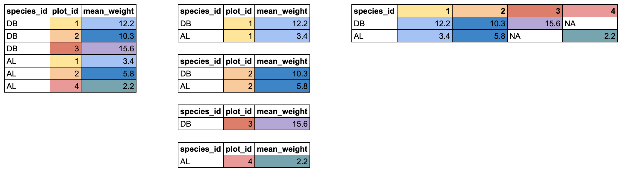 {alt='Diagram depicting the behavior of
 pivot_wider() on a small tabular dataset.'}
In our case, we want the new columns to be named from our plot_id column, with the values coming from the mean_weight column. We can pipe our data.frame right into pivot_wider() and add those two arguments:
sp_by_plot_wide <- sp_by_plot %>%
  pivot_wider(names_from = plot_id,
              values_from = mean_weight)

sp_by_plot_wide
## # A tibble: 18 × 25
## # Groups:   species_id [18]
##    species_id    `3`   `21`    `1`    `2`    `4`   `5`    `6`   `7`    `8`
##    <chr>       <dbl>  <dbl>  <dbl>  <dbl>  <dbl> <dbl>  <dbl> <dbl>  <dbl>
##  1 BA           8      6.5   NA     NA     NA     NA    NA     NA    NA
##  2 DM          41.2   41.5   42.7   42.6   41.9   42.6  42.1   43.2  43.4
##  3 DO          42.7   NA     50.1   50.3   46.8   50.4  49.0   52    49.2
##  4 DS         128.    NA    129.   125.   118.   111.  114.   126.  128.
##  5 NL         171.   136.   154.   171.   164.   192.  176.   170.  134.
##  6 OL          32.1   28.6   35.5   34     33.0   32.6  31.8   NA    30.3
##  7 OT          24.1   24.1   23.7   24.9   26.5   23.6  23.5   22    24.1
##  8 OX          22     NA     NA     22     NA     20    NA     NA    NA
##  9 PE          22.7   19.6   21.6   22.0   NA     21    21.6   22.8  19.4
## 10 PF           7.12   7.23   6.57   6.89   6.75   7.5   7.54   7     6.78
## 11 PH          28     31     NA     NA     NA     29    NA     NA    NA
## 12 PM          20.1   23.6   23.7   23.9   NA     23.7  22.3   23.4  23
## 13 PP          17.1   13.6   14.3   16.4   14.8   19.8  16.8   NA    13.9
## 14 RF          14.8   17     NA     16     NA     14    12.1   13    NA
## 15 RM          10.3    9.89  10.9   10.6   10.4   10.8  10.6   10.7   9
## 16 SF          NA     49     NA     NA     NA     NA    NA     NA    NA
## 17 SH          76.0   79.9   NA     88     NA     82.7  NA     NA    NA
## 18 SS          NA     NA     NA     NA     NA     NA    NA     NA    NA
## # ℹ 15 more variables: `9` <dbl>, `10` <dbl>, `11` <dbl>, `12` <dbl>,
## #   `13` <dbl>, `14` <dbl>, `15` <dbl>, `16` <dbl>, `17` <dbl>, `18` <dbl>,
## #   `19` <dbl>, `20` <dbl>, `22` <dbl>, `23` <dbl>, `24` <dbl>
Now we've got our reshaped data.frame. There are a few things to notice. First, we have a new column for each plot_id value. There is one old column left in the data.frame: species_id. It wasn't used in pivot_wider(), so it stays, and now contains a single entry for each unique species_id value.
Finally, a lot of NAs have appeared. Some species aren't found in every plot, but because a data.frame has to have a value in every row and every column, an NA is inserted. We can double-check this to verify what is going on.
Looking in our new pivoted data.frame, we can see that there is an NA value for the species BA in plot 1. Let's take our sp_by_plot data.frame and look for the mean_weight of that species + plot combination.
sp_by_plot %>%
  filter(species_id == "BA" & plot_id == 1)
## # A tibble: 0 × 3
## # Groups:   species_id [0]
## # ℹ 3 variables: species_id <chr>, plot_id <dbl>, mean_weight <dbl>
We get back 0 rows. There is no mean_weight for the species BA in plot 1. This either happened because no BA were ever caught in plot 1, or because every BA caught in plot 1 had an NA weight value and all the rows got removed when we used filter(!is.na(weight)) in the process of making sp_by_plot. Because there are no rows with that species + plot combination, in our pivoted data.frame, the value gets filled with NA.
There is another pivot_ function that does the opposite, moving data from a wide to long format, called pivot_longer(). It takes 3 arguments: cols for the columns you want to pivot, names_to for the name of the new column which will contain the old column names, and values_to for the name of the new column which will contain the old values.
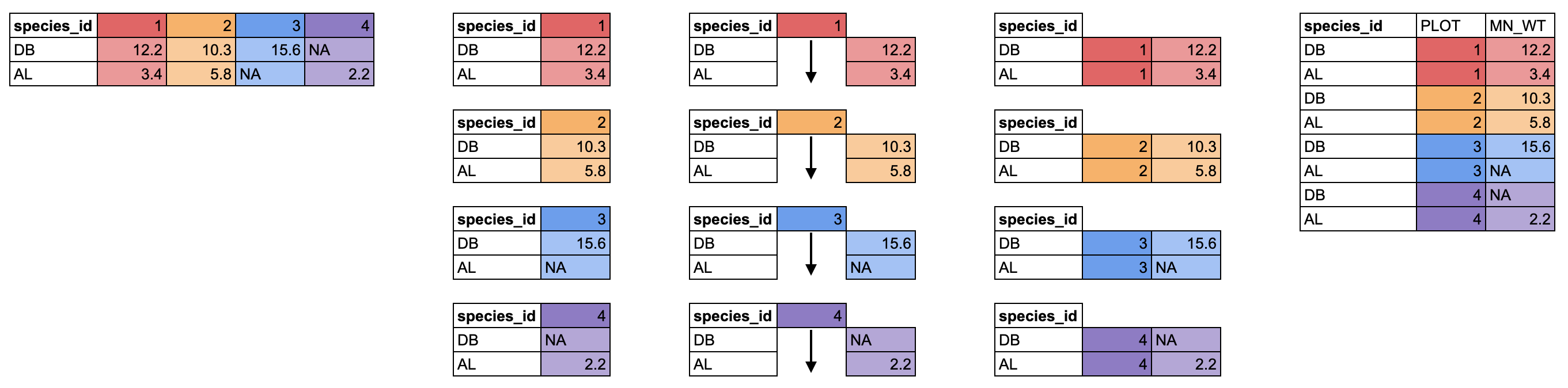 {alt='Diagram depicting the behavior of
 pivot_longer() on a small tabular dataset.'}
We can pivot our new wide data.frame to a long format using pivot_longer(). We want to pivot all the columns except species_id, and we will use PLOT for the new column of plot IDs, and MEAN_WT for the new column of mean weight values.
sp_by_plot_wide %>%
  pivot_longer(cols = -species_id, names_to = "PLOT", values_to = "MEAN_WT")
## # A tibble: 432 × 3
## # Groups:   species_id [18]
##    species_id PLOT  MEAN_WT
##    <chr>      <chr>   <dbl>
##  1 BA         3         8
##  2 BA         21        6.5
##  3 BA         1        NA
##  4 BA         2        NA
##  5 BA         4        NA
##  6 BA         5        NA
##  7 BA         6        NA
##  8 BA         7        NA
##  9 BA         8        NA
## 10 BA         9        NA
## # ℹ 422 more rows
One thing you will notice is that all those NA values that got generated when we pivoted wider. However, we can filter those out, which gets us back to the same data as sp_by_plot, before we pivoted it wider.
sp_by_plot_wide %>%
  pivot_longer(cols = -species_id, names_to = "PLOT", values_to = "MEAN_WT") %>%
  filter(!is.na(MEAN_WT))
## # A tibble: 300 × 3
## # Groups:   species_id [18]
##    species_id PLOT  MEAN_WT
##    <chr>      <chr>   <dbl>
##  1 BA         3         8
##  2 BA         21        6.5
##  3 DM         3        41.2
##  4 DM         21       41.5
##  5 DM         1        42.7
##  6 DM         2        42.6
##  7 DM         4        41.9
##  8 DM         5        42.6
##  9 DM         6        42.1
## 10 DM         7        43.2
## # ℹ 290 more rows
Data are often recorded in spreadsheets in a wider format, but lots of tidyverse tools, especially ggplot2, like data in a longer format, so pivot_longer() is often very useful.
Getting rid of any row where any value is NA with drop_na()
In the split-apply-combine approach section above, we covered how to remove NA values for a specific column.
If instead of removing NAs from a single column you would like to drop any row where any column is an NA, you can use the drop_na() function.
surveys %>%
  drop_na()
## # A tibble: 13,773 × 13
##    record_id month   day  year plot_id species_id sex   hindfoot_length weight
##        <dbl> <dbl> <dbl> <dbl>   <dbl> <chr>      <chr>           <dbl>  <dbl>
##  1        63     8    19  1977       3 DM         M                  35     40
##  2        64     8    19  1977       7 DM         M                  37     48
##  3        65     8    19  1977       4 DM         F                  34     29
##  4        66     8    19  1977       4 DM         F                  35     46
##  5        67     8    19  1977       7 DM         M                  35     36
##  6        68     8    19  1977       8 DO         F                  32     52
##  7        69     8    19  1977       2 PF         M                  15      8
##  8        70     8    19  1977       3 OX         F                  21     22
##  9        71     8    19  1977       7 DM         F                  36     35
## 10        74     8    19  1977       8 PF         M                  12      7
## # ℹ 13,763 more rows
## # ℹ 4 more variables: genus <chr>, species <chr>, taxa <chr>, plot_type <chr>
Alternatively, you can provide column names to the drop_na() function to specify which columns to remove NA values from.
surveys %>%
  drop_na(hindfoot_length, weight)
## # A tibble: 13,797 × 13
##    record_id month   day  year plot_id species_id sex   hindfoot_length weight
##        <dbl> <dbl> <dbl> <dbl>   <dbl> <chr>      <chr>           <dbl>  <dbl>
##  1        63     8    19  1977       3 DM         M                  35     40
##  2        64     8    19  1977       7 DM         M                  37     48
##  3        65     8    19  1977       4 DM         F                  34     29
##  4        66     8    19  1977       4 DM         F                  35     46
##  5        67     8    19  1977       7 DM         M                  35     36
##  6        68     8    19  1977       8 DO         F                  32     52
##  7        69     8    19  1977       2 PF         M                  15      8
##  8        70     8    19  1977       3 OX         F                  21     22
##  9        71     8    19  1977       7 DM         F                  36     35
## 10        74     8    19  1977       8 PF         M                  12      7
## # ℹ 13,787 more rows
## # ℹ 4 more variables: genus <chr>, species <chr>, taxa <chr>, plot_type <chr>
Tidy selection
In the select section above, we demonstrated how to select columns based on column name.
You can select columns based on whether they match a certain criteria by using tidyselect functions.
Below, we'll demonstrate how to use the where() function and the ends_with() function, but there are many additional tidyselect functions such asstarts_with()orcontains()`.
With the where() function, we can select columns that match a specific conditions.
If we want all numeric columns, we can ask to select all the columns where the class is numeric:
select(surveys, where(is.numeric))
## # A tibble: 16,878 × 7
##    record_id month   day  year plot_id hindfoot_length weight
##        <dbl> <dbl> <dbl> <dbl>   <dbl>           <dbl>  <dbl>
##  1         1     7    16  1977       2              32     NA
##  2         2     7    16  1977       3              33     NA
##  3         3     7    16  1977       2              37     NA
##  4         4     7    16  1977       7              36     NA
##  5         5     7    16  1977       3              35     NA
##  6         6     7    16  1977       1              14     NA
##  7         7     7    16  1977       2              NA     NA
##  8         8     7    16  1977       1              37     NA
##  9         9     7    16  1977       1              34     NA
## 10        10     7    16  1977       6              20     NA
## # ℹ 16,868 more rows
Instead of giving names or positions of columns, we instead pass the where() function with the name of another function inside it, in this case is.numeric(), and we get all the columns for which that function returns TRUE.
We can use this to select any columns that have any NA values in them:
select(surveys, where(anyNA))
## # A tibble: 16,878 × 7
##    species_id sex   hindfoot_length weight genus       species  taxa
##    <chr>      <chr>           <dbl>  <dbl> <chr>       <chr>    <chr>
##  1 NL         M                  32     NA Neotoma     albigula Rodent
##  2 NL         M                  33     NA Neotoma     albigula Rodent
##  3 DM         F                  37     NA Dipodomys   merriami Rodent
##  4 DM         M                  36     NA Dipodomys   merriami Rodent
##  5 DM         M                  35     NA Dipodomys   merriami Rodent
##  6 PF         M                  14     NA Perognathus flavus   Rodent
##  7 PE         F                  NA     NA Peromyscus  eremicus Rodent
##  8 DM         M                  37     NA Dipodomys   merriami Rodent
##  9 DM         F                  34     NA Dipodomys   merriami Rodent
## 10 PF         F                  20     NA Perognathus flavus   Rodent
## # ℹ 16,868 more rows
Instead of matching on a condition, the ends_with() function match variables (in this case column names) according to a given pattern.
We'll use the string "_id" to select columns that end with the string _id: record_id, plot_id, and species_id.
select(surveys, ends_with("_id"))
## # A tibble: 16,878 × 3
##    record_id plot_id species_id
##        <dbl>   <dbl> <chr>
##  1         1       2 NL
##  2         2       3 NL
##  3         3       2 DM
##  4         4       7 DM
##  5         5       3 DM
##  6         6       1 PF
##  7         7       2 PE
##  8         8       1 DM
##  9         9       1 DM
## 10        10       6 PF
## # ℹ 16,868 more rows
More on joining data together with dplyr
We briefly covered how to join two data.frames together above. If you would like more information and practice doing joins, this lesson provides more information and practice. It relies on a similar data set to the one we've been using in this lesson.